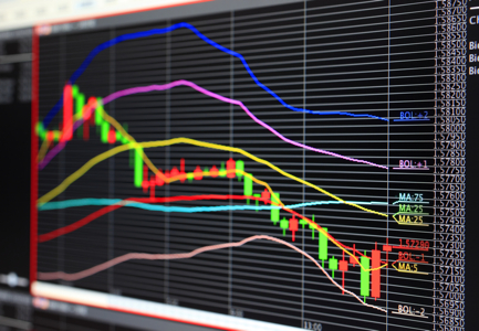
Foreign exchange market chart
Li, Hoi, Zhao, and Gopalkrishnan (2012), from Nanyang Technological University, Singapore, and the Deloitte Analytics Institute (Asia), Singapore, developed a very sophisticated algorithm for portfolio selection that they labelled the “Confidence Weighted Mean Reversion” (CWMR) strategy. The principle of mean reversion in portfolio selection is to invest in stocks that performed poorly during the previous period. The portfolio is long-only and, therefore, simply avoids stocks that have performed well in the previous period, rather than shorting them. CWMR is a machine-learning algorithm that responded to both the mean and the variance of the portfolio, and strove to always maintain a Gaussian, or normal, distribution.
The CWMR strategy was tested on eight extensive data sets, with daily data from 1962 to 2011, as well as intraday and weekly data. The data sets included stocks from NYSE, the Toronto Stock Exchange (TSE), as well as a collection of global stock indices (MSCI). Intraday data came from the DJIA 30 and NASDAQ 100 stocks.
Given the complexity of the data sets, the authors determined to test six versions of the CWMR strategy by comparing them to 13 other strategies. These included:
- Buy and hold;
- Select the best individual stock (or index) from the data set (a hindsight strategy);
- Best constant rebalanced portfolio (a hindsight strategy);
- And ten other algorithmic methods proposed by other researchers in previously published studies.
The experimental tests measured the cumulative wealth attained by each strategy at the end of the data period.
The result was described by the authors as “somehow beyond imagination.” The CWMR algorithms dominated the competition, in all instances but two. Typically, the cumulative wealth achieved by the CWMR strategy, in daily data series, was many multiples better than either of the two hindsight methods. Particularly notable were the intraday tests in which the trades issued by the CWMR strategies achieved success ratios exceeding 63%.
Further analysis indicated that these results could be sustained with transaction costs and that drawdowns were reasonable in comparison to other methods.
Li and Hoi (2012) submitted a paper with yet another machine-learning, mean-regression algorithm that they labeled the “online learning moving average reversion” (OLMAR) strategy. In a series of tests very similar to those reported above, they reported that OLMAR even outperformed the CWMR strategy.
Li, Zhao, Hoi, and Gopalkrishnan (2012) reported on yet another algorithm that they label the “passive aggressive mean reversion” (PAMR) strategy. This strategy attained a very high level of performance, comparable with those previously mentioned. Furthermore, the data set and MatLab source codes have been made available online at http://www.cais.ntu.edu.sg/~chhoi/PAMR/.
Trading strategy: This strategy requires a team with the resources and knowledge to implement these unique artificial intelligence applications. The research cited suggests that the potential payoff would justify the investment.